Note
Go to the end to download the full example code.
Basic usage
This example shows the basic operation on the nikamap.NikaMap object
Generate fake map
from fake_map import create_dataset

create_dataset()
Read the data
By default the read routine will read the 1mm band, but any band can be read
Note
This fake dataset as been generated by the fake_map.py script
data_path = os.getcwd()
nm = NikaMap.read(os.path.join(data_path, "fake_map.fits"))
NikaMap is derived from the astropy.NDData class and thus you can access and and manipulate the data the same way
nm.data: an np.array containing the brightnessnm.wcs: a WCS object describing the astrometry of the imagenm.uncertainy.array: a np.array containing the uncertainty arraynm.mask: a boolean mask of the observationsnm.meta: a copy of the header of the original map
print(nm)
[[nan nan nan ... nan nan nan]
 [nan nan nan ... nan nan nan]
 [nan nan nan ... nan nan nan]
 ...
 [nan nan nan ... nan nan nan]
 [nan nan nan ... nan nan nan]
 [nan nan nan ... nan nan nan]] Jy / beam
print(nm.wcs)
WCS Keywords

Number of WCS axes: 2
CTYPE : 'RA---TAN' 'DEC--TAN'
CUNIT : 'deg' 'deg'
CRVAL : 0.0 0.0
CRPIX : 255.5 255.5
PC1_1 PC1_2  : 1.0 0.0
PC2_1 PC2_2  : 0.0 1.0
CDELT : -0.00055555555555556 0.00055555555555556
NAXIS : 512  512
NikaMap objects support slicing like numpy arrays, thus one can access part of the dataset
print(nm[96:128, 96:128])
[[-6.33690088e-04  1.69940188e-05  1.13807169e-02 ... -4.77849898e-04
  -4.42656104e-03  1.29046581e-03]
 [-2.72178236e-03 -3.45859875e-03  6.88742228e-03 ... -1.64266145e-03
  -2.13449370e-04  1.42029957e-03]
 [-1.61883365e-03 -1.94432669e-03  6.59878990e-03 ... -5.03622493e-03
  -3.17169283e-03 -1.80714630e-03]
 ...
 [-2.25541455e-03  7.91104592e-03 -7.27016993e-03 ... -4.20066714e-03
  -1.19154754e-03 -2.18287246e-04]
 [-5.37531694e-04 -1.29236258e-03 -2.83427495e-03 ...  5.39804507e-03
   1.34197023e-03  2.60073558e-03]
 [ 3.62899719e-03  2.33734785e-03 -3.51804099e-04 ... -2.20487005e-03
   2.53243571e-03  3.69477925e-03]] Jy / beam
Basic Plotting
thus they can be plotted directly using maplotlib routines
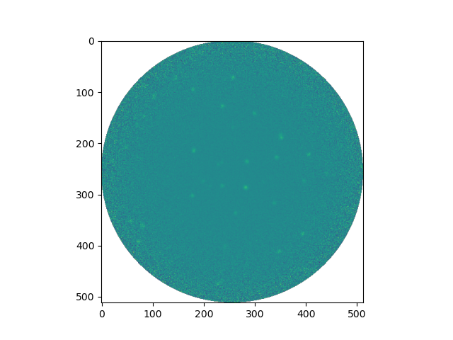
<matplotlib.image.AxesImage object at 0x7f0ff91266d0>
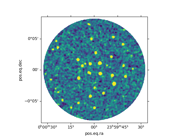
or using the convience routine of nikamap.NikaMap
<matplotlib.image.AxesImage object at 0x7f0ffa5f8910>
nm.plot_SNR(cbar=True)

<matplotlib.image.AxesImage object at 0x7f0ffa637c90>
or the power spectrum density of the data :
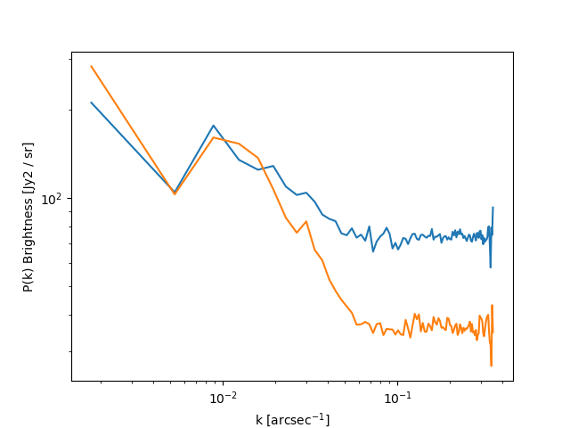
Beware that these PSD are based on an non-uniform noise, thus dominated by the largest noise part of the map
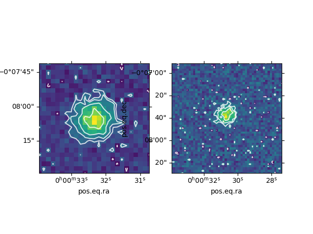
Match filtering
A match filter algorithm can be applied to the data to improve the detectability of sources. Here using the gaussian beam as the filter
mf_nm = nm.match_filter(nm.beam)
mf_nm.plot_SNR()
<matplotlib.image.AxesImage object at 0x7f0ffa4c3790>
Source detection & photometry
A peak finding algorithm can be applied to the SNR datasets
mf_nm.detect_sources(threshold=3)
/home/abeelen/bin/miniconda3/envs/nikamap/lib/python3.11/site-packages/gwcs/__init__.py:61: UserWarning: pkg_resources is deprecated as an API. See https://setuptools.pypa.io/en/latest/pkg_resources.html. The pkg_resources package is slated for removal as early as 2025-11-30. Refrain from using this package or pin to Setuptools<81.
  from pkg_resources import get_distribution, DistributionNotFound
The resulting catalog is stored in the sources property of the nikamap.NikaMap object
print(mf_nm.sources)
 ID  id x_peak ...         _ra                   _dec
               ...         deg                   deg
--- --- ------ ... -------------------- ---------------------
  0  47    282 ...   359.98471141224087  0.017900473325902548
  1  34    284 ...    359.9833680530288  -0.01023494570515759
  2  27    181 ...  0.04103657758760216 -0.022078623176958436
  3  24    352 ...    359.9461055682787  -0.03665709100734357
  4  31    342 ...    359.9511180377267 -0.014897141134770702
  5  45    236 ...  0.01013188779160079  0.016091643955198284
  6  48    178 ...   0.0426365060967777  0.026824391340317215
  7  16    237 ... 0.009989964144739918  -0.07051554696883071
  8  17    299 ...    359.9751664481243  -0.06253307235182007
... ...    ... ...                  ...                   ...
 57  63    208 ... 0.025873658457146263   0.08891158255812076
 58  51    132 ...  0.06783594831038264    0.0417855909726289
 59   5    321 ...    359.9630533237226  -0.10488540846597848
 60  30     71 ...   0.1018934447849608 -0.014997892881757482
 61  60    290 ...    359.9802965664621   0.07864611766770525
 62  23     80 ...  0.09679655906523227  -0.04605940596994251
 63   3    336 ...    359.9550290799297  -0.12365226677175188
 64  15    408 ...   359.91481364554465  -0.07074167149134783
 65   4    314 ...   359.96703294799136  -0.10753079786957036
 66   2    174 ...  0.04466632155317542  -0.12341022916464929
Length = 67 rows
and can be overploted on the SNR maplotlib
mf_nm.plot_SNR(cat=True)
<matplotlib.image.AxesImage object at 0x7f0ff822b350>
There is two available photometries : * peak_flux : to retrieve point sources flux directly on the pixel value of the map, ideadlly on the matched filtered map * psf_flux : which perfom psf fitting on the pixels at the given position
mf_nm.phot_sources(peak=True, psf=False)
catalog which can be transfered to the un-filtered dataset, where psf fitting can be performed
nm.phot_sources(sources=mf_nm.sources, peak=False, psf=True)
the sources attribute now contains both photometries
print(nm.sources)
 ID  id x_peak y_peak ... group_id        qfit                 cfit
                      ...
--- --- ------ ------ ... -------- ------------------ ---------------------
  0  47    282    287 ...        1  8.152994922178257  0.059939660029874484
  1  34    284    236 ...        2  12.64336869618628 0.0002133592185613038
  2  27    181    215 ...        3 13.366328594585362  -0.07895493616234243
  3  24    352    189 ...        4 18.413140379387276    0.1181550258600761
  4  31    342    228 ...        5 16.334757054331373  -0.43033140210881426
  5  45    236    283 ...        6 18.605298897451014  -0.35911451755184826
  6  48    178    303 ...        7 17.251515749291965 -0.018264574198010593
  7  16    237    128 ...        8 19.383464894150322 -0.020089576715589127
  8  17    299    142 ...        9 23.203284893541138   -0.4694455084491426
... ...    ...    ... ...      ...                ...                   ...
 57  63    208    414 ...       50 124.58698856463074   -0.3708325300772956
 58  51    132    330 ...       51 143.64314111386796    0.2082426810258432
 59   5    321     66 ...       52 155.32444002862704    -1.949814307892258
 60  30     71    227 ...       41  243.1493969749096    0.7388320662456204
 61  60    290    396 ...       53 157.53088130538507   -0.6386854332702907
 62  23     80    172 ...       29  168.0524948107374    1.2417805970251061
 63   3    336     32 ...       54   147.154185985862    2.2274796199782947
 64  15    408    127 ...       34 145.74316805380448  -0.14035328637361438
 65   4    314     61 ...       52  154.9876641149034    1.8956788406675709
 66   2    174     32 ...       55 155.62012408444818    2.0765425347606907
Length = 67 rows
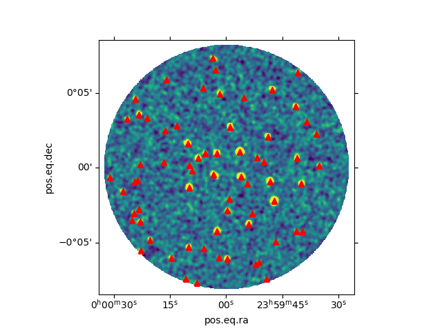
which can be compared to the original fake source catalog
fake_sources = Table.read("fake_map.fits", "FAKE_SOURCES")
fake_sources.meta["name"] = "fake sources"
nm.plot_SNR(cat=[(fake_sources, {"marker": "^"}), (nm.sources, {"marker": "+"})])
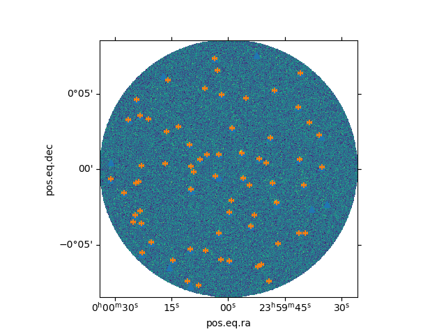
<matplotlib.image.AxesImage object at 0x7f0fe3fb4c10>
or in greater details :
fake_coords = SkyCoord(fake_sources["ra"], fake_sources["dec"], unit="deg")
detected_coords = SkyCoord(nm.sources["ra"], nm.sources["dec"], unit="deg")

idx, sep2d, _ = fake_coords.match_to_catalog_sky(detected_coords)
good = sep2d < 10 * u.arcsec
idx = idx[good]
sep2d = sep2d[good]

ra_off = Angle(fake_sources[good]["ra"] - nm.sources[idx]["ra"], "deg")
dec_off = Angle(fake_sources[good]["dec"] - nm.sources[idx]["dec"], "deg")

fig, axes = plt.subplots(ncols=2)
for method in ["flux_psf", "flux_peak"]:
    axes[0].errorbar(
        fake_sources[good]["amplitude"],
        nm.sources[idx][method],
        yerr=nm.sources[idx]["e{}".format(method)],
        fmt="o",
        label=method,
    )
axes[0].legend(loc="best")
axes[0].set_xlabel("input flux [mJy]")
axes[0].set_ylabel("detected flux [mJy]")

axes[1].scatter(ra_off.arcsecond, dec_off.arcsecond)
axes[1].set_xlabel("R.A. off [arcsec]")
axes[1].set_ylabel("Dec. off [arcsec]")
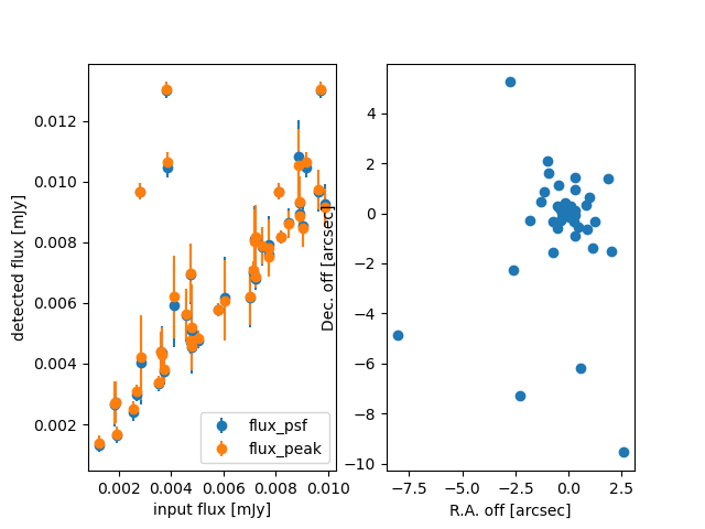
Text(305.89267676767673, 0.5, 'Dec. off [arcsec]')
Total running time of the script: (0 minutes 2.859 seconds)