---

This example shows how to use the three noise-estimation classes HalfDifference, Jackknife and Bootstrap on a set of synthetic single-scan FITS files.

Each class reads a list of per-scan maps (in IDL/NIKA2 pipeline FITS format), combines them and produces noise realisations whose SNR distribution should be Gaussian with unit standard deviation.

All three classes inherit from MultiScans and are usable as callables and as iterators.

import tempfile
from pathlib import Path

import astropy.units as u
import matplotlib.pyplot as plt
import numpy as np
from astropy.io import fits
from astropy.modeling import models
from astropy.nddata import StdDevUncertainty
from astropy.stats.funcs import gaussian_fwhm_to_sigma
from astropy.table import Table
from astropy.wcs import WCS
from photutils.datasets import make_model_image

from nikamap import Bootstrap, ContMap, HalfDifference, Jackknife, NikaMap

rng = np.random.default_rng(42)

Build synthetic per-scan FITS files

We simulate 100 independent scans of the same field: each scan has uniform coverage, a Gaussian noise level of 1 mJy/beam and a 12.5″ FWHM beam. Three faint point sources are embedded in each scan at SNR ≈ 1 per scan; they reach SNR ≈ 10 in the co-added map. The files are written in IDL pipeline FITS format (the format read by NikaMap by default).

shape = (64, 64)
pixscale = 3 * u.arcsec
fwhm = 12.5 * u.arcsec
noise_level = 1  # mJy/beam  (per scan)
n_scans = 100

wcs = WCS(naxis=2)
wcs.wcs.crpix = [shape[1] / 2, shape[0] / 2]
wcs.wcs.cdelt = [-pixscale.to("deg").value, pixscale.to("deg").value]
wcs.wcs.crval = [0.0, 0.0]
wcs.wcs.ctype = ["RA---TAN", "DEC--TAN"]
img_header = wcs.to_header()
img_header["UNIT"] = "Jy / beam"

primary_header = fits.Header()
primary_header["f_sampli"] = 10.0, "[Hz] sampling frequency"
primary_header["FWHM_260"] = fwhm.to(u.arcsec).value, "[arcsec] beam FWHM at 1mm"
primary_header["FWHM_150"] = fwhm.to(u.arcsec).value, "[arcsec] beam FWHM at 2mm"

hits = np.ones(shape, dtype=int) * 100
stddev = np.full(shape, noise_level)

# Build the static signal: 3 point sources each with peak = noise_level
# (SNR≈1 per scan, SNR≈10 in the 100-scan co-add)
beam_std_pix = (fwhm / pixscale).decompose().value * gaussian_fwhm_to_sigma
source_table = Table(
    {
        "x_mean": [16.0, 44.0, 28.0],
        "y_mean": [16.0, 32.0, 48.0],
        "amplitude": [noise_level, noise_level, noise_level],
        "x_stddev": [beam_std_pix, beam_std_pix, beam_std_pix],
        "y_stddev": [beam_std_pix, beam_std_pix, beam_std_pix],
        "theta": [0.0, 0.0, 0.0],
    }
)
signal = make_model_image(shape, models.Gaussian2D(), source_table,
                          model_shape=shape, x_name="x_mean", y_name="y_mean")

tmpdir = Path(tempfile.mkdtemp())
filenames = []
for i in range(n_scans):
    noise = rng.normal(0, noise_level, size=shape)
    hdus = fits.HDUList(
        [
            fits.PrimaryHDU(header=primary_header),
            fits.ImageHDU(noise + signal, header=img_header, name="Brightness_1mm"),
            fits.ImageHDU(stddev, header=img_header, name="Stddev_1mm"),
            fits.ImageHDU(hits, header=img_header, name="Nhits_1mm"),
        ]
    )
    fname = tmpdir / f"scan_{i:02d}.fits"
    hdus.writeto(fname)
    filenames.append(fname)

print(f"Created {len(filenames)} scan files in {tmpdir}")

Created 100 scan files in /tmp/tmpymw80wmw

Weighted co-add (baseline)

All three classes can be used as callables. When instantiated with n=None (the default for HalfDifference and Jackknife) they return the straightforward inverse-variance weighted co-add of all scans. The three embedded sources are clearly visible in this map.

hd = HalfDifference(filenames, n=None)
coadd = hd()
print("Co-add SNR σ:", coadd.check_SNR_simple())

Co-add SNR σ: 1.042829438419616

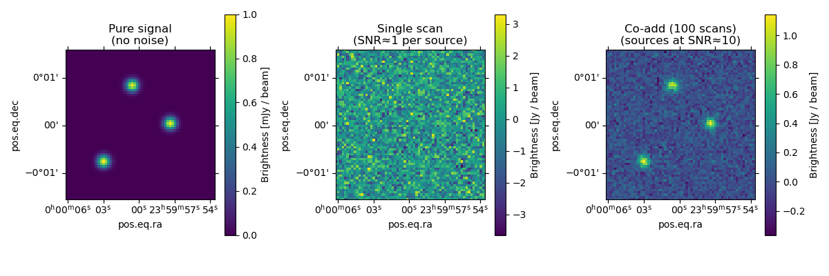
Signal and single-scan maps

The pure signal map shows the three embedded point sources with no noise. A single scan buries those sources under noise (SNR ≈ 1 per source). After co-adding all 100 scans the sources emerge at SNR ≈ 10.

signal_cm = ContMap(
    signal,
    uncertainty=StdDevUncertainty(stddev),
    wcs=wcs,
    unit=u.mJy / u.beam,
)
one_scan_map = NikaMap.read(filenames[0])

fig, axes = plt.subplots(1, 3, figsize=(12, 4), subplot_kw={"projection": coadd.wcs})
for ax, nm, title in zip(
    axes,
    [signal_cm, one_scan_map, coadd],
    ["Pure signal\n(no noise)", "Single scan\n(SNR≈1 per source)", "Co-add (100 scans)\n(sources at SNR≈10)"],
):
    nm.plot(ax=ax, cbar=True)
    ax.set_title(title)
fig.tight_layout()

HalfDifference — signal-free noise maps

HalfDifference assigns random ±1 weights to scans and computes the weighted sum. Because equal numbers of scans receive +1 and -1 weights, astrophysical signal cancels exactly while the noise accumulates in the same way as in the co-add: the resulting uncertainty map is identical to the co-add uncertainty (no √2 penalty).

The map therefore contains only noise — the sources present in each scan are not visible — and the SNR distribution should be Gaussian with unit standard deviation (σ ≈ 1).

Pass n to set how many realisations the iterator will yield.

hd = HalfDifference(filenames, n=5)

# Using it as a callable returns one realisation
hd_map = hd()

Using it as an iterator yields n independent realisations

hd_snr_stds = [nm.check_SNR_simple() for nm in HalfDifference(filenames, n=5)]
print("HalfDifference SNR σ:", [f"{s:.3f}" for s in hd_snr_stds])

HalfDifference SNR σ: ['0.978', '1.016', '0.994', '0.973', '0.992']

Jackknife — sub-sample variance noise maps

Jackknife partitions the scans into n_samples groups, computes the inter-group variance as the noise estimate and returns the weighted mean of the groups. Like HalfDifference, signal cancels in the inter-group differences so the resulting map is noise-only. Increasing n_samples improves the degrees of freedom of the variance estimator; with n_samples=10 there are 9 degrees of freedom.

jk = Jackknife(filenames, n_samples=100, n=5)
jk_map = jk()
jk_snr_stds = [nm.check_SNR_simple() for nm in Jackknife(filenames, n_samples=10, n=5)]
print("Jackknife      SNR σ:", [f"{s:.3f}" for s in jk_snr_stds])

INFO: overwriting masked ndarray's current mask with specified mask. [astropy.nddata.nddata]
INFO: overwriting masked ndarray's current mask with specified mask. [astropy.nddata.nddata]
INFO: overwriting masked ndarray's current mask with specified mask. [astropy.nddata.nddata]
INFO: overwriting masked ndarray's current mask with specified mask. [astropy.nddata.nddata]
INFO: overwriting masked ndarray's current mask with specified mask. [astropy.nddata.nddata]
INFO: overwriting masked ndarray's current mask with specified mask. [astropy.nddata.nddata]
Jackknife      SNR σ: ['1.062', '1.049', '1.073', '1.074', '1.090']

Bootstrap — resampled noise maps

Bootstrap resamples the scan list with replacement n_bootstrap times. The pixel-wise standard deviation of the resampled co-adds gives the empirical uncertainty, while their mean is returned as the signal map. It is the most computationally expensive option but makes no assumption about the per-scan noise distribution.

Bootstrap is a callable (not an iterator): a single call returns the bootstrapped mean map whose uncertainty is the bootstrap std. The default n_bootstrap is 50 × n_scans; here we use a smaller value suitable for a quick example.

bs = Bootstrap(filenames, n_bootstrap=200)
bs_map = bs()
print("Bootstrap      SNR σ:  ", f"{bs_map.check_SNR_simple():.3f}")

Bootstrap      SNR σ:   1.159

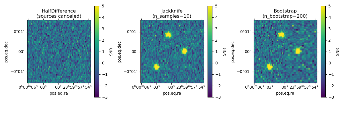
Visual comparison of the SNR maps

The co-add clearly shows the three embedded sources. The three noise maps (HalfDifference, Jackknife, Bootstrap) should be featureless: sources cancel because the same signal is present in every scan.

fig, axes = plt.subplots(1, 3, figsize=(12, 4), subplot_kw={"projection": hd_map.wcs})
for ax, nm, title in zip(
    axes,
    [hd_map, jk_map, bs_map],
    [
        "HalfDifference\n(sources canceled)",
        "Jackknife\n(n_samples=10)",
        "Bootstrap\n(n_bootstrap=200)",
    ],
):
    nm.plot_SNR(ax=ax, cbar=True)
    ax.set_title(title)
fig.tight_layout()

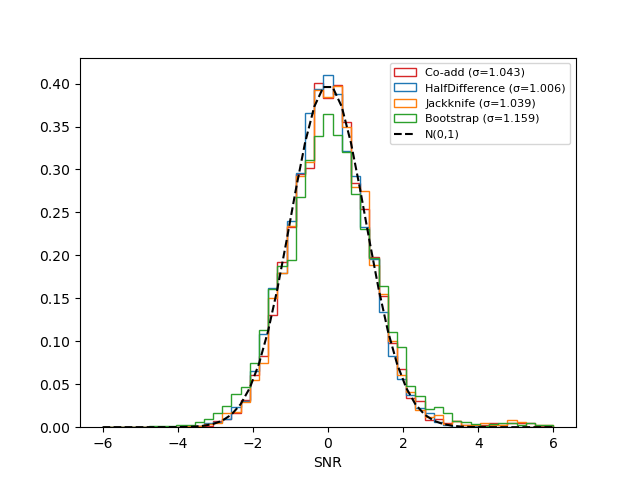
SNR histogram comparison

The noise maps (HalfDifference, Jackknife, Bootstrap) should all produce SNR distributions consistent with N(0, 1). The co-add histogram is wider because of the source peaks; the noise maps histograms should match N(0, 1) closely (σ ≈ 1).

import scipy.stats as spstats

fig, ax = plt.subplots()
bins = np.linspace(-6, 6, 50)
for nm, label, color in zip(
    [coadd, hd_map, jk_map, bs_map],
    ["Co-add", "HalfDifference", "Jackknife", "Bootstrap"],
    ["C3", "C0", "C1", "C2"],
):
    snr = nm.snr.compressed()
    sigma = nm.check_SNR_simple()
    ax.hist(snr, bins=bins, density=True, histtype="step", color=color,
            label=f"{label} (σ={sigma:.3f})")
ax.plot(bins, spstats.norm.pdf(bins), "k--", lw=1.5, label="N(0,1)")
ax.set_xlabel("SNR")
ax.legend(fontsize=8)

plt.show()

Cleanup temporary files

import shutil

shutil.rmtree(tmpdir)