Simultaneous stacking (simstack)

Recover the mean flux of source populations via linear regression on the map.

Simstack (Viero et al. 2013) fits a linear combination of beam-convolved hit maps — one per source population — directly to the map pixel values. Unlike sequential cutout stacking, it simultaneously solves for all populations and therefore removes the cross-contamination between spatially correlated groups.

This example demonstrates simstack() on a synthetic ContMap with two source populations of known flux.

import astropy.units as u
import matplotlib.pyplot as plt
import numpy as np
from astropy.coordinates import SkyCoord
from astropy.modeling import models
from astropy.nddata import StdDevUncertainty
from astropy.stats.funcs import gaussian_fwhm_to_sigma
from astropy.table import Table
from astropy.wcs import WCS
from photutils.datasets import make_model_image

from nikamap import ContBeam, ContMap

rng = np.random.default_rng(42)

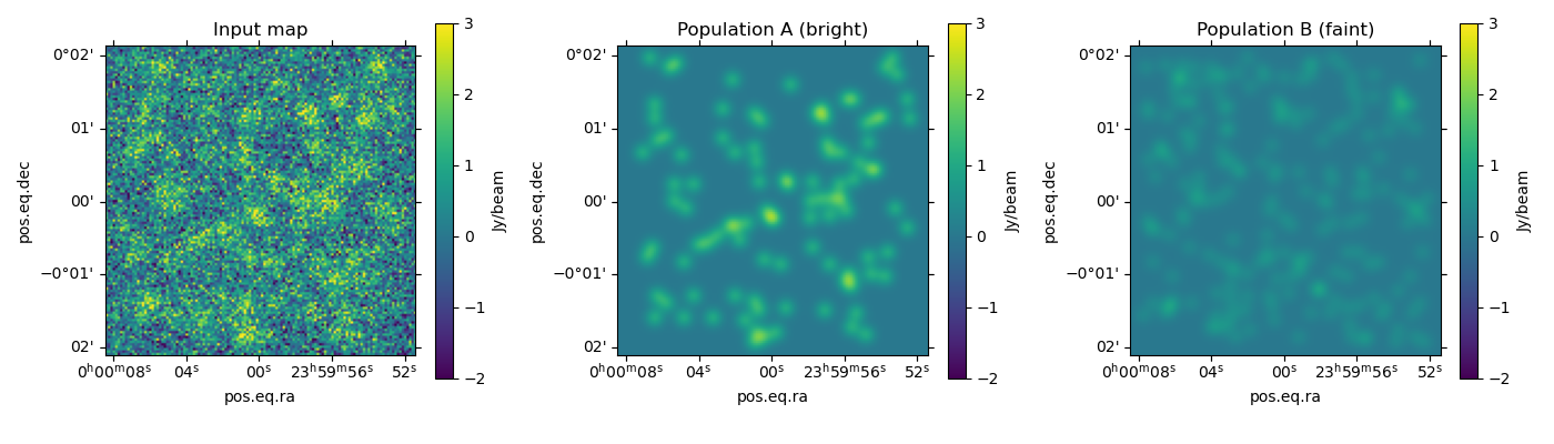
Build a synthetic map with two source populations

• Population A — 100 “bright” sources at 1 mJy/beam

• Population B — 200 “faint” sources at 0.3 mJy/beam

Both populations are unresolved (beam = 12.5″ FWHM, pixel = 2″).

shape = (128, 128)
pixscale = 2 * u.arcsec
fwhm = 12.5 * u.arcsec
noise_level = 1  # mJy/beam

flux_A = 1  # mJy/beam
flux_B = 0.3  # mJy/beam
nsrc_A = 100
nsrc_B = 200

wcs = WCS(naxis=2)
wcs.wcs.crpix = [shape[1] / 2, shape[0] / 2]
wcs.wcs.cdelt = [-pixscale.to("deg").value, pixscale.to("deg").value]
wcs.wcs.crval = [0.0, 0.0]
wcs.wcs.ctype = ["RA---TAN", "DEC--TAN"]

beam_std_pix = (fwhm / pixscale).decompose().value * gaussian_fwhm_to_sigma


def _make_source_table(nsources, flux, margin=5):
    x = rng.integers(margin, shape[1] - margin, nsources).astype(float)
    y = rng.integers(margin, shape[0] - margin, nsources).astype(float)
    return Table(
        {
            "x_mean": x,
            "y_mean": y,
            "amplitude": np.full(nsources, flux),
            "x_stddev": np.full(nsources, beam_std_pix),
            "y_stddev": np.full(nsources, beam_std_pix),
            "theta": np.zeros(nsources),
        }
    )


table_A = _make_source_table(nsrc_A, flux_A)
table_B = _make_source_table(nsrc_B, flux_B)

map_A = make_model_image(shape, models.Gaussian2D(), table_A,
                         model_shape=shape, x_name="x_mean", y_name="y_mean")
map_B = make_model_image(shape, models.Gaussian2D(), table_B,
                         model_shape=shape, x_name="x_mean", y_name="y_mean")

noise_map = rng.normal(0, noise_level, size=shape)

cm = ContMap(
    map_A + map_B + noise_map,
    uncertainty=StdDevUncertainty(np.full(shape, noise_level)),
    wcs=wcs,
    unit=u.mJy / u.beam,
    beam=ContBeam(major=fwhm, pixscale=pixscale),
)

Convert pixel positions to sky coordinates

coords_A = SkyCoord(wcs.pixel_to_world(table_A["x_mean"], table_A["y_mean"]))
coords_B = SkyCoord(wcs.pixel_to_world(table_B["x_mean"], table_B["y_mean"]))

Single-population simstack

When coords is a single SkyCoord, the method returns the mean flux and 1-sigma uncertainty of that one population.

flux_fit_A, err_fit_A = cm.simstack(coords_A)
print(
    f"Population A — injected: {flux_A:.1f} mJy/beam  " f"recovered: {flux_fit_A[0]:.2f} ± {err_fit_A[0]:.2f} mJy/beam"
)

Population A — injected: 1.0 mJy/beam  recovered: 1.21 ± 0.02 mJy/beam

Multi-population simstack

Passing a list of SkyCoord solves for all populations simultaneously. Each element of the list defines one population; the returned arrays have one entry per population.

fluxes, errs = cm.simstack([coords_A, coords_B])

print(f"Population A — injected: {flux_A:.1f} mJy/beam  " f"recovered: {fluxes[0]:.2f} ± {errs[0]:.2f} mJy/beam")
print(f"Population B — injected: {flux_B:.1f} mJy/beam  " f"recovered: {fluxes[1]:.2f} ± {errs[1]:.2f} mJy/beam")

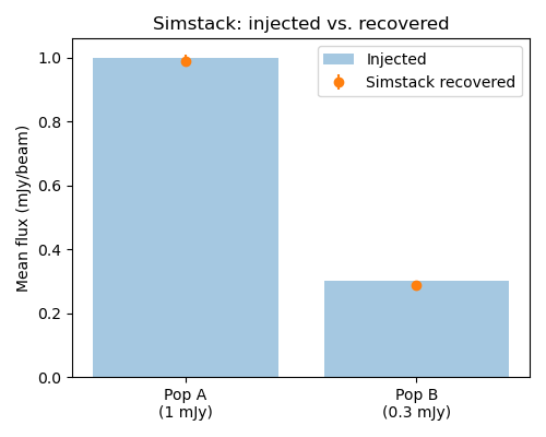
Population A — injected: 1.0 mJy/beam  recovered: 0.99 ± 0.02 mJy/beam
Population B — injected: 0.3 mJy/beam  recovered: 0.29 ± 0.01 mJy/beam

Add a constant offset term

If the map has a residual DC level, pass add_offset=True to absorb it into the fit. The offset coefficient is appended at the end of the arrays.

fluxes_off, errs_off = cm.simstack([coords_A, coords_B], add_offset=True)
print(f"With offset — Population A: {fluxes_off[0]:.2f} ± {errs_off[0]:.2f} mJy/beam")
print(f"With offset — Population B: {fluxes_off[1]:.2f} ± {errs_off[1]:.2f} mJy/beam")
print(f"Fitted offset             : {fluxes_off[2] * 1e3:.1f} µJy/beam")

With offset — Population A: 0.99 ± 0.02 mJy/beam
With offset — Population B: 0.28 ± 0.01 mJy/beam
Fitted offset             : 5.2 µJy/beam

Visualise

fig, axes = plt.subplots(1, 3, figsize=(14, 4),
                          subplot_kw={"projection": cm.wcs})

labels = ["Input map", "Population A (bright)", "Population B (faint)"]
sub_maps = [cm.data, map_A, map_B]
for ax, data, title in zip(axes, sub_maps, labels):
    im = ax.imshow(data, origin="lower", vmin=-2 * noise_level, vmax=3 * noise_level)
    ax.set_title(title)
    plt.colorbar(im, ax=ax, label="Jy/beam")

plt.tight_layout()

Summary plot — recovered vs. injected fluxes

fig, ax = plt.subplots(figsize=(5, 4))
populations = ["Pop A\n(1 mJy)", "Pop B\n(0.3 mJy)"]
injected = np.array([flux_A, flux_B])
recovered = np.array([fluxes[0], fluxes[1]])
errors = np.array([errs[0], errs[1]])

ax.bar(populations, injected, alpha=0.4, label="Injected")
ax.errorbar(populations, recovered, yerr=errors, fmt="o", color="C1",
            label="Simstack recovered", zorder=5)
ax.set_ylabel("Mean flux (mJy/beam)")
ax.set_title("Simstack: injected vs. recovered")
ax.legend()
plt.tight_layout()